Running NORMA 
NORMA basics
The main program of the NORMA software suite is a simplex minimization code
with optional simulated annealing, which is provided as a pre-compiled executable named NORMA.exe.
All minimization parameters can be defined by the user in the input parameter file
NORMA.inp,
that will be read by NORMA.exe at start-up (for details on the available parameters see below).
NORMA.exe communicates with URO and the NMA code via a short script called func.sh.
This script performs a single minimization step.
It reads the normal mode amplitudes for the actual minimization step
from a file func.in, that has been generated by NORMA.exe.
func.sh then generates a new normal mode perturbed structure, fits this
structure into the EM density using URO, and eventually writes the corresponding misfit parameter Q to
a file func.out.
This file is then read by NORMA.exe in order to determine the
amplitudes for the next minimization step.
All computations are performed in a sub-directory named RUN.minimize.
This directory may be renamed to save a successful NORMA run.
The following flowchart displays this approach and lists the different scripts
that are involved.
NORMA flowchart
NORMA.exe --> writes amplitudes to file func.in   (Format: MODE1 DQ1 ... MODEn DQn)

NORMA.exe --> calls func.sh as a shell process

              func.sh --> reads amplitudes from func.in

              func.sh --> calls script pert_multi_mode.sh (NMA)

                          pert_multi_mode.sh --> calls pdbmat (elastic network computation)
                                             --> calls diagrtb (computes normal modes)
                                             --> calls proj_mod (generates a perturbed model)

              func.sh --> calls script go.URO.minimize

                          go.URO.minimize    --> calls URO programs (i.e. fitting)
                                             --> gets misfit Q from URO output

              func.sh --> writes misfit Q to file func.out (Format: Q*1000, Integer)

NORMA.exe --> reads misfit Q from file func.out
              and computes next set of amplitudes
Running NORMA on a new case
The easiest way to get an idea on how NORMA works, is to run the GroEl example
on your own and play with some of the parameters.
Briefly, to create and run a new case with NORMA, setup URO using the following command
csh $URO/setup
This will generate a number of files and directories that will be used by URO.
Then move your structure file (PDB format) and the electron density map (EZD format) to the ./d
directory (this directory is created by the above setup command).
The structure should be roughly placed inside the EM map.
Also in the ./d directory, generate the symmetry files (sym
& gs.sym) and the file containing the symmetries to be used by URO
(symlist).
Refer to the URO documentation for details.
In the simple case where only one copy of the structure file needs to be fitted, these symmetry related files can be simply copied from
the Ca-ATPase example. For higher order symmetries, refer to the tools provided by URO.
Place a copy of the files func.sh
and go.URO.minimize in the main directory.
Adapt the names of the PDB file and the file containing the EM-density in the first lines
of these scripts (e.g. pdb=1aonA.pdb and map=GroEl.ezd).
Type NORMA.exe to start the fitting process.
NORMA input parameters
As already mentioned above, the behavior of the minimizer can be parameterized using
a file named NORMA.inp. This file (actually a FORTRAN NAMELIST file) has the following
format:
&PARAM
 NDIM    = 3,            ! nnumber of normal modes to use for fitting
 MODE    = 7 8 9,        ! modes to use (starting with 7 for the lowest frequency mode)
 PB      = 0.  0.  0.,   ! initial guess of the amplitudes
 DY      = 200.,         ! expected amplitude range
 NITER   = 50,           ! number of iterations of a single minimization run
 TEMPTR  = 50.,          ! "temperature" of the simulated annealing scheme
 NANNEAL = 0,            ! number of simulated annealing steps (0 = no annealing)
 NROUND  = 1,            ! number of minimization rounds
 LRAND   = F,            ! randomization of initial perturbations
 TOL     =  1E-3,        ! relative tolerance for convergence
 SEED    =  42.4710999,  ! initial random seed
 NVERB   = 1             ! verbosity level
/
NORMA dumps all parameters in this format upon start-up, so you can verify the actual default
parameters at that moment, and you can check whether your parameters have been taken into account correctly.
If no file NORMA.inp is present, NORMA uses its default values.
In the NORMA.inp any parameter that is not specified will take its default value.
Here is an example of a NORMA.inp file.
|
Example 1: GroEl
The objective of this example is to fit the open form of a single GroEl molecule into
the electron density of the GroEl complex in its closed form.
First, we will describe the software side of the problem.
Then, we will discuss results obtained using different fitting parameters.
Finally, we will give some suggestions for advanced protocols.
The following publications describe the different structures and electron microscopy data that are used here.
1AON, open form: Ranson NA, Farr GW, Roseman AM, Gowen B, Fenton WA, Horwich AL, Saibil HR.,
ATP-bound states of GroEL captured by cryo-electron microscopy.
, Cell. 2001; 107:869-879.
1SX3, closed form: Chaudhry C, Horwich AL, Brunger AT, Adams PD.,
Exploring the structural dynamics of the E.coli chaperonin GroEL using translation-libration-screw crystallographic refinement of intermediate states.
, J. Mol. Biol. 2004; 342:229-245.
GroEl electron microscopy: De Carlo S, El-Bez C, Alvarez-Rua C, Borge J, Dubochet J.,
Cryo-negative staining reduces electron-beam sensitivity of vitrified biological particles.
, J. Struct. Biol. 2002; 138:216-226.
Setting up of the GroEl case
The GroEl case is part of the NORMA distribution and is installed (and eventually tested) in the
NORMA-1.0/groel directory. However, in order to start from scratch, all data
required for the GroEl case can also be downloaded in a separate file
example1.tgz, that can then be extracted anywhere to a new directory by
tar xvfz example1.tgz
This wil extract the the following files to a sub-directory called example1. This directory contains the following files:
- GroEl.ezd
- The GroEl EM density map in NEWEZD format.
- 1aonA.pdb
- The initial model, open conformation, positioned in the EM map.
- Aa.1SX3.pdb
- PDB file of the closed conformation, positioned in the EM map.
- gs.sym - sym
- Two files containing the symmetry operators imposed on the
EM reconstruction: gs.sym (O format) and sym (URO format).
The URO script o2u.scr can be used to transform an (O format) file into an
URO type symmetry file (see URO documentation).
- symlist
- The list of those symmetry operators that are defined in the sym file and that shall be used in the fitting.
- gs.real
- The initial O view (only required for viewing with O). This file can be create using the command write .gs_real in O.
Note that NORMA will run correctly without this file.
- NORMA.inp
- The input parameter for the minimization.
- func.sh
- A shell script that computes the function to minimize. It will be called by NORMA.exe
and reads a file func.in as input. It will output a file func.out containing the value
of the function to be minimized, that is, the misfit parameter Q.
In fact, we multiply Q by a factor of 1000 for convenience (to avoid real arithmetics at the Unix shell level).
- func.in
- This file contains the list of normal modes and the corresponding amplitudes that shall be applied when
the script func.sh is called.
This file will be overwritten by NORMA.exe - it is only provided here for testing purposes.
- go.URO.minimize
- The shell script that calls the URO programs. It is called by the script func.sh.
Enter the example1 directory and setup the URO files by typing
cd ./example1
csh $URO/setup
This will copy a number of URO files to the current directory, and generate three sub-directories
./d, ./e, and ./i.
Move the following files to the ./d directory by typing
mv sym gs.sym gs.real symlist GroEl.ezd 1aonA.pdb Aa.1SX3.pdb ./d
Now, everything is ready for the minimization.
Type
NORMA.exe
to start the minimization.
After running NORMA, you can use the utility script gen_pert.sh to
compute a PDB file for an animated view of the fitting process.
Typing
gen_pert.sh 7 -575
will compute 11 instances of the fitted structure in a file anim.pdb, using a perturbation following mode 7
with an amplitude varying between 0 and -575 (the optimal amplitude for this example when using
a single normal mode). This file can be viewed as an animated by using for example VMD.
If all works correctly, here is what you should see:
NORMA example output
You should obtain the same result when running the test.sh script in the NORMA directory as follows:
./test.sh groel
However, if this is the first case you
run NORMA, chances are that some errors slip in somewhere.
If this happens, the first place to look at is the file
func.log. All error messages that are generated by the func.sh
script will be directed to this file.
If the problem seems to be related to URO itself,
you may enter the sub-directory RUN.minimize.
This directory is regenerated every time the script go.URO.minimize is called.
From inside this directory you can call all URO programs, just as if you were using
URO interactively.
Check the files emft.log, scat1.log, and fit.log for error messages.
If the problem seems to be related to the normal mode computation, or to the interaction
of the different NORMA scripts, you can run one step of the minimization by typing sh ./func.sh.
Make sure that the file func.in exists.
Check the files pdbmat.log, diagrtb.log, and proj_modes.log for error messages.
If all works correctly, the file func.out should contain an integer number (Q*1000).
Fitting GroEl with different parameters
Once the technical problems solved, the next question is how to find the optimal fitting parameters.
That is, how many and which modes should be used? What amplitude range do we start with? Is the result robust
under change of these parameters, or does the fitting get trapped in a local minimu?
In order to get an idea of the normal modes properties of the protein, a first step is to submit its structure to the
elNémo web server.
Here is the result of such a submission for the GroEl open form (1aon). As we also know the closed form in this case,
we can ask elNémo to compute the projection of the normal modes onto the closed form of GroEl (1sx3):
elNémo:
click here to see elNémo computation for GroEl 1AON projected onto 1SX3
Below are the final amplitudes after fitting of the open form of GroEl (1aon)
into the electron density map of the closed form, using a different number of
normal modes and different initial conditions:
Fit of GroEl 1AON using different modes:
  Mode   DQ(1)   DQ(3)    DQ(5)    DQ(10)      PROJ
    7    568.5   590.0    520.4     459.1     566.5
    8           -139.2   -40.67      82.6      40.7
    9            -42.6    129.0     118.7      27.1
   10                    -230.5    -312.5     137.5
   11                    -113.7     -86.4    -310.6
   12                              -189.1     -16.1
   13                               -39.7      15.5
   14                                22.3     100.2
   15                                70.3     -38.9
   16                               455.7    -101.3
- DQ(5) was initialized using the results from DQ(3);
- DQ(10) was initialized using the results from DQ(5)+;
- DQ(12) was initialized using the results from DQ(10);
- PROJ is the projection of 1AON onto 1SX3 (see
elNémo)
The corresponding values of the correlation coefficient (CC), R-factor (R), and misfit (Q)
are given below. The root mean square distance (RMSD) with respect to the closed form (1sx3) was
computed using LSQMAN. To check how well the closed form of GroEl (1sx3) fits the EM densiry,
a NORMA fitting using 12 modes was also performed.
                             CC     R     Q      RMSD
1SX3               #         85.3  68.6  13.8     ref
1SX3_fit 12 modes  #         87.7  64.3  11.6   2.955

1AON               #         61.5  78.5  32.7  11.965
1AON_fit 1  mode   #         76.0  76.2  21.5   7.923
1AON_fit 3  modes  #         76.5  76.6  21.0   7.505
1AON_fit 5  modes  #         78.8  74.6  19.1   5.849
1AON_fit 10 modes  #         83.3  66.6  15.4   9.345
We note that 1sx3 fits quite well into the EM density, although some improvement can still be made.
A fit of the open form (1aon) using a single mode drastically improves the fit (Q drops from 32.7 to 21.5),
while also reducing the RMSD with respect to the closed form (RMSD drops from 11.965 to 7.923).
Using 3 modes only yields moderate improvement, while using 5 modes can still improve the fit.
This is coherent with the projection of 1aon onti 1sx3 using elNémo,
that is mode 7 (lowest non-trivial mode) and mode 11 (5th non-trivial mode) contribute
most to the conformational change between the opened and the closed structure (with an amplitude of DQ=566.5 and DQ=-310.6, respectively).
Using 10 modes still allows to decrease the misfit parameter (Q), but at the cost of an increasing RMSD.
The following animations of the fitting process clearly show that using 10 modes leads to an overfitting in this case.
From the topview it becomes clear that the 5 mode fit is also less optimal than it appears
(black structure: 1SX3_fit using 12 modes).
In the next chapter we will discuss an advanced protocol, that actually allows
a complete flexible fit of the open form of GroEl into the EM density.
Advanced fitting protocols
Apparently, a fitting in a single steps leads to unrealistic solutions (trapping in
a local minimum?). Now we take a multi-step approach as follows:
- Step 1
- Fit starting with 1aon using a single mode (mode 7).
- Step 2
- Application of 30% of the amplitude computed for a best fit from step 1.
Idealization of the resulting structure using REFMAC. Fit starting with this model, again using
only mode 7.
- Step 3
- Application of 50% of the amplitude computed for a best fit from step 2.
Idealization of the resulting structure using REFMAC. Fit starting with this model, again using
only mode 7.
- Step 4
- Application of 100% of the amplitude computed for a best fit from step 3.
Idealization of the resulting structure using REFMAC. Fit starting with this model, again using
the 12 lowest frequency modes.
                                                                          CC    RF     Q
          ref   : 1aon unperturbed                                    #  61.5  78.5  32.7
animation step 1: starting with 1aon, using 1 mode                    #  76.0  76.2  21.5
animation step 2: starting with 1aon.30.ideal, using 1 mode           #  77.6  74.6  20.1
animation step 3: starting with 1aon.30.50.ideal, using 1 mode        #  79.7  73.4  18.5
animation step 4: starting with 1aon.30.50.100.ideal, using 12 modes  #  82.8  69.7  15.9
(click on the animation links to see the fitting of the individual steps).
Animated view of GroEl 1AON using this 4 step fitting:
groel4step.avi (AVI-Format)
|